Accessing Your Algorithm’s ‘Statistical API’

From linear and logistic regressions, tree-based algorithms and SVM to standard neural networks, they all focus on one thing: optimization. Their inherent goal is to optimise the gap between predictions and observed data with the good old loss function and techniques like gradient descent paving the way.

But probability is not optimization. Indeed, if we want to use the language of statistics to describe our models in terms of their relationships between parameters, features and target, what do we do? What’s the trick that’ll lift our model into a probabilistic domain?

Well as it turns out there’s a ‘statistical API’ that can expose some tools to us to do just this (fyi, I’ll probably be burnt at the stake by statistical purists for tainting hallowed ground with that analogy 🔥).

But before we get there, let’s take a linear regression and look at its core target when it comes to optimisation…

The error term

The error term, ε, the mathematical embodiment of all the residuals, is what our linear regression’s loss function focuses on minimizing so it can optimise the difference between predictions and observed data. But, if we assume this error term consists of residuals that don’t influence one another and that follow the same statistical distribution (i.e. they’re independent and identically distributed (i.i.d)), we can start expanding our horizons.

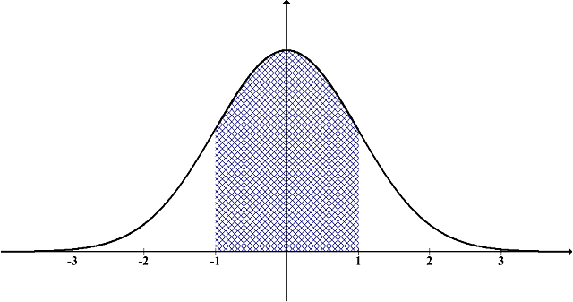
That is, under i.i.d assumptions, we can assume the error term follows a specific statistical distribution. In linear regression we typically assume a Gaussian (Normal) distribution of the error term. This stems from the Central Limit Theorem (CLT). That is, regardless of the population’s underlying distribution, we know via the CLT that if we were to take a large enough amount of random samples, calculate the mean for each and plot these means we would see a distribution converging on Gaussian. Similarly, we can assume that if we were to draw the residuals and plot the sample means of the errors they would converge on a Gaussian distribution, hence its application.

Getting probabilistic

Now we’ve constrained the error term to a specific distribution we can leverage the distribution’s probability density function (PDF), or probability mass function (PMF) for discrete outcomes. And this is the pivotal step because, as the ‘P’ in PDF and PMF suggests, we finally bring those elusive probabilities into play.

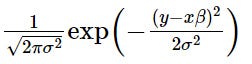
To give you some feel for this, let’s examine the mathematical expression for the PDF of a Gaussian distribution as applied to linear regression:

**(Note, please see the end of the article for a more detailed examination of this and its link to the to-be-discussed MLE¹)

The main focus in the above equation is y — xβ. To quickly explain this, let’s take a look at the generalised matrix form for linear regression:

Here,

• y is what we’re trying to predict, our target (or response variable)
• xβ (or ŷ) is effectively expressing the process of summing the product of our features (or predictors) with their respective weights, plus the intercept, to make a prediction of y.
• ε is our error term i.e. all the differences between what we’re trying to predict and our predictions.

From this, we can now see that the y — xβ bit in our Gaussian PDF is just the error term, ε. And that means when we construct the PDF its x-axis can be interpreted as being centred on our predicted value, ŷ (xβ), with the variation around it horizontally capturing the model’s variance i.e. the degree of error between predicted and observed values, y. Thus, for any given y, this allows us to calculate the density under the PDF curve between it and ŷ (we say y is conditioned on ŷ). Mathematically, this equates to calculating the related integral, which tells us the likelihood of observing an value within that range under the assumed model. Of course, a similar process exists for the PMF, but as you have a discrete variable you find the ‘mass’ via summation, not integration.

Anyway, through this density or mass calculation, we’re then in a position to determine what is known as the likelihood function, which relates to the conditional probability of P(observed data | parameters) — where ‘|’ means ‘given’. Furthermore, by finding the values of our parameters (intercept, weights and variance) that maximise the likelihood of observing the given data, we arrive at the Maximum Likelihood Estimation (MLE).

A quick recap

So, we started with our basic optimisation goal, as per the loss function. By throwing in a few nifty assumptions — in the case of linear regression with respect to the error term — we’ve managed to transition into a probabilistic space. A space that, courtesy of our ‘statistical API’, exposes to us the likelihood function, the conditional P(observed data | parameters), and, by extension, the MLE, which finds the parameter values that maximises this probability.

How neat is that! 🥳

Unleash the (incredibly important) nuance

The ‘likelihood’, the conditional probability we’ve just discussed, belongs to the statistical paradigm/philosophy known as Frequentism. By that I mean, the frequency (hence Frequentism) of our random sampling is what leads to convergence between the observed data and the population parameters — theoretically, infinite random samples are needed to ensure perfect congruence.

e.g. Flipping a coin

A Frequentist approach to flipping a fair coin would be to give the likelihood as the probability of getting our observed data (random samples of some size) given the parameter of, say, landing heads (0.5). Now, obviously, if we take 10 or 1 billion random samples (that’s going to be one tired thumb) we can’t ever guarantee a perfect 50/50 split (we might get lucky, but we can’t ensure it). What Frequentism tells us though is the more random samples we take the more we’ll see the data move in the direction of our parameters (btw, this property is known as the Law of Large Numbers).

Now, here comes one of most critical bits of Frequentism: the observed data is what varies/is probabilistic; the population parameters are fixed (be they known or unknown).

*Please let the nuance of that last sentence really sink in if this is new to you.

Consequently, when we’re dealing with the likelihood function or Frequentism in general we can’t speak of or quantify our algorithm’s level of uncertainty in its parameters because, fundamentally, they’re set in stone so no probabilities exist for them.

But what do we do if we do want this probabilistic insight into our model’s parameters?

For our API’s next trick…

Thankfully, our ‘statistical API’ doesn’t end there in its functionality. It exposes us to just the probability we want thanks to Bayes’ Theorem. What follows is a beautiful link between our algorithm, Frequentism and the other big statistical paradigm/philosophy, Bayesianism:

***(Note, the above is a simplification, please see the end of the article if you’re interested in the equation’s full form²)

Of course, the first probability in the numerator is the likelihood, our Frequentist conditional probability.

P(parameters) is known as the ‘prior’. Priors relate to Bayesian statistics and they represent our pre-existing beliefs about the parameters. Obviously, beliefs like “Matthew needs to get out more😆” aren’t probabilities, they’re just a collection of words. That’s why, like we did with our loss function, we need to express them using a statistical distribution (Gaussian, Binomial, Beta, Exponential etc.) based on which one we think is most suitable. This step then allows us to describe them probabilistically (you’re probably seeing a pattern by now).

P(observed data) is known as the ‘evidence’ or ‘marginal likelihood’. It is the probability of observed data given the features (predictors), integrated over the entire parameter space.

Mathematically, the evidence serves as a normalising constant for the numerator so the conditional probability can be expressed as a valid probability distribution. In reality, this is a very tricky beast to calculate precisely. It goes rapidly from a computational nightmare to intractable as the parameter space increases in dimensionality, basically for each parameter we add we’re nesting an integral within another😱 Thankfully, various clever workarounds are available to estimate it instead — Markov Chain Monte Carlo (MCMC) being a common example. I should also mention here that if the distribution for our prior comes from the same family as the one for the likelihood then we can have a ‘conjugate prior’, and the maths is such that the marginal likelihood can be ignored — handy right! Sadly though, a lot of real-world scenarios don’t lend themselves readily to conjugate priors.

Anyway, let’s move on to the remaining component of the equation because that’s where the magic happens.

A Bayesian ta-da✨

Remember we wanted a way to describe/quantify our algorithm’s level of uncertainty in the parameters given Frequentism’s limits? Well, in a puff of smoke it has appeared. P(parameters | observed data), commonly known as the ‘posterior’, does just this!

That is, given its Bayesian nature, it treats the observed data as fixed and the parameters as variable/probabilistic. Additionally, it departs from the Frequentist focus on the frequency of random sampling. Instead, it takes an iterative approach that acknowledges two things: one, our beliefs about the world guide how probable we think something is going to be; two, as we’re exposed to new data, we update our beliefs accordingly.

Of course, you can see the posterior’s incorporation of belief via the prior. And it’s for this reason that Bayesian modelling allows us to build in existing domain knowledge/expertise. It should be noted here that some people argue this introduces an element of subjectivity that could be problematic. But, nevertheless, because Bayesian modelling isn’t dependent on the principle of lots of random sampling, if you have an informative prior and very little data to work with, this approach can be a particularly good choice.

Pretty cool right!

Frequentist vs. Bayesian approaches

Often these two paradigms are pitted against one another and some people choose to actively identify themselves with one or the other. Personally, I see pros and cons in each and a place for both in terms of what they can do and say — something I hope this article has given a little glimpse into.

What is vital is that the nuances between the two are properly understood; otherwise, issues can quickly rear their head. On this note and as a last case in point, I give you the Frequentist ‘confidence level’ and ‘confidence interval’, and the Bayesian ‘credible interval’.

The former is widely used and, by virtue of our ‘statistical API’, becomes another probability-related tool with which to describe our model. But its definition needs precision:

For a given confidence level of x% we can say that, with a large number of repeated random samples, the probability of the confidence intervals containing the fixed population parameter will show convergence on x/100.

As you’ll notice, this definition articulates the Frequentist idea of large amounts of random sampling, which when theoretically infinite would yield perfect convergence with the population parameter. Also, via the confidence interval, it stresses probability in terms of the observed data, not the fixed parameters.

By the way, be careful here not to fall into the trap of incorrectly ascribing the confidence level to a given confidence interval — the confidence level is in relation to all random samples.

Compare this with the definition of a Bayesian credible interval:

Based on the data and prior beliefs, there’s an x% probability that the population parameter lies within the interval.

Note, no mention of repeated sampling. Also, we’re incorporating prior knowledge and, this time, we’re talking about the probability of the parameter (probabilistic) lying within the given interval (fixed), not across multiple intervals.

Anyway, I just wanted to hammer home these differences, so they could be appreciated.

Wrapping this API up

So, there we have it. Our ‘statistical API’ has connected our optimization algorithm to the statistical domain. It has exposed powerful Frequentist and Bayesian tools that enable us to describe our model’s observed data and parameters in nuanced, probabilistic ways. And all without a ‘GET’ request in sight!

(Note, if you’d like a more in-depth article on anything presented here or other subjects please let me know.)

[1] Likelihood function to MLE (as applies to linear regression):

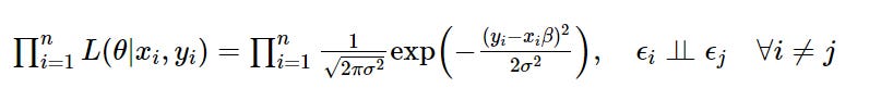
Here, the connection is expressed between the likelihood function (L) and the PDF equation with the condition that the error term follows a Gaussian distribution made explicit.

To find the parameters, θ, that maximise the likelihood as per MLE we begin by taking the product of the probabilities over the entire PDF (which is only allowed because we have independency as per our i.i.d assumption of the error term). This finds the joint probability i.e. the likelihood of all the observed data:

To simplify we can then take the natural log:

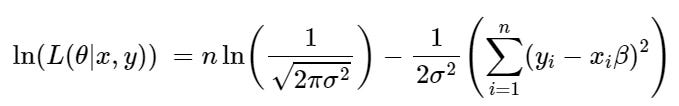
Now we can take the partial derivatives of the log likelihood function with respect to each parameter in the parameter space, which for linear regression is the intercept, weights and variance.

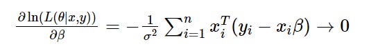
E.g. Partial derivative with respect to β set to zero to calculate the optimal value with respect to the MLE:

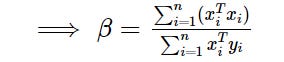
Of course, this is only identifying a turning point for β at the moment. To establish whether it is maximal we would have to examine the related Hessian matrix. This uses good old eigenvectors to establish the direction of the curvature in vector space and the related eigenvalues indicate the nature of the curvature by their sign (negative = maximum, mixed negative and positive = saddle, positive = minimum).

(Update: Someone wanted me to expand on this last point, so I will briefly)

The second partial derivative for the log-likelihood function with respect to β transpose and β is:

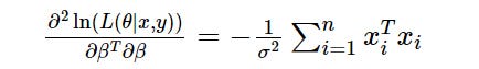
However, to construct the associated Hessian matrix you would normally calculate the second partial derivative with respect to each term in the β vector. Thankfully, in this scenario, these derivatives will all be in the same above form and, as there no interdependencies courtesy of our i.i.d. assumption, all the off-diagonal values in the matrix will, handily, be zero:

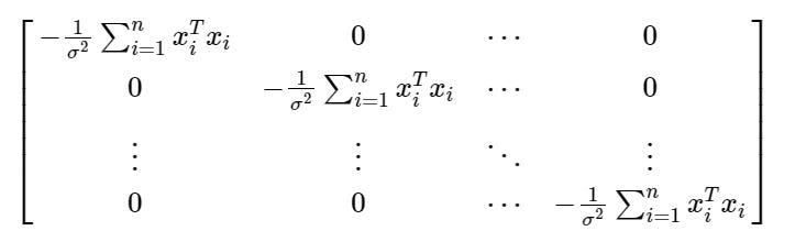
Now, given that we’ve got a diagonal matrix, the eigenvalues are simply the values on the diagonal. And, given that we’re effectively multiplying each element of the matrix ‘x’ by itself, we’ll always have a positive number yielded by the summation which, in turn, will always be made negative by the constant. Therefore, each eigenvalue is negative implying concavity and that we have indeed found a maximum! It’s a bit involved I know but, at the very least, it’s worth having an idea of the concepts at play.

[2] Bayes’ Theorem for linear regression:

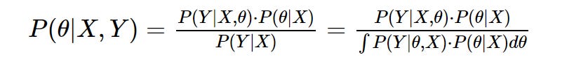
Y = observed data, X = feature space (predictors) and θ = parameter space (incl. intercept, weights and variance).

Where, for instance, P(θ|X,Y) is read as the probability of the parameters given the joint probability of the feature space and observed data.

This version of the equation more clearly describes the relationship between the observed values, feature space and parameters. Moreover, we see the way in which the ‘evidence’ involves calculating the integral over the entire parameter space for the product of the likelihood and prior (which, it should be noted, is just the joint probability of Y, θ and X partially expanded by the chain rule).

More content at PlainEnglish.io.

Sign up for our free weekly newsletter. Follow us on Twitter, LinkedIn, YouTube, and Discord.

---

Accessing Your Algorithm’s ‘Statistical API’ was originally published in Artificial Intelligence in Plain English on Medium, where people are continuing the conversation by highlighting and responding to this story.

https://ai.plainenglish.io/accessing-your-algorithms-statistical-api-928357507792?source=rss—-78d064101951—4
By: Matthew
Title: Accessing Your Algorithm’s ‘Statistical API’
Sourced From: ai.plainenglish.io/accessing-your-algorithms-statistical-api-928357507792?source=rss—-78d064101951—4
Published Date: Wed, 28 Jun 2023 02:02:01 GMT

Did you miss our previous article…
https://e-bookreadercomparison.com/langchain-streamlit-llama-bringing-conversational-ai-to-your-local-machine/