Validation of Parametric Short-term Strategies with Python: How Fast Can You Really Go?

Introduction

In this article, the goal is to find the most efficient method in Python for calculating the backtest of a parametric model. Model validation tools that are sufficiently robust require evaluating objective functions across a very large parameter space and on datasets representing at least 20 years of data. It is vital for a researcher to find the most suitable computational framework so that their creativity is not hindered by excessively long computation times.

Parametric models:

A parametric model is a model that depends on a data set and on a set of parameters.

These parameters have predefined values that determine the model’s combination space, which is represented by all possible n_plet combinations [p1, p2….pn].

Each of these unique n_plets generates a specific trading signal, and every signal corresponds to a particular value of the fitness function, which we select to calibrate the model.

Calibrating the model involves identifying the n_plet that maximizes the fitness function across the parameter space.

For instance, a very basic seasonal model in which every day I open a trade at a specific hour and close it at another specific hour, is described by 2 parameters: the entry hour and the exit hour, and the parameter space is formed by all the pairs (T entry, T exit).

If we assume the instruments trades 23 hours every day, there are 23*22 possible pairs or 2_plets.

Validating a model always implies to generate a Matrix that encompasses all the time series of returns associated with the parametric space. The number of columns in this Matrix is equivalent to the total possible parameter combinations (e.g., 23*22 in the previous simple example). Meanwhile, the number of rows is determined by the number of timestamps in the return time series.

For instance, suppose we have ten years of price observations, and each year has 250 trading days. In that case, the number of columns in the Matrix would be (250*10)-1 (excluding one because the calculation transitions from price to return).

Path dependent and non-path dependent parametric models:

For what will follow it is important to define two subclasses of parametric models: path-dependent and non-path-dependent models.

Path-dependent model: In this type of strategy, the entry and exit conditions are determined based on the current or previous trades. The decision-making process depends on the historical trading activity and the progression of trades.

Example: A strategy that uses a trailing stop loss order is path dependent. The stop loss level is adjusted based on the performance of the trade, such as locking in profits or limiting losses. The exit decision depends on the specific path the trade takes and is influenced by the trade’s performance over time.

Non-path-dependent model: a non-path-dependent strategy in the context of systematic trading refers to an approach where the entry and exit decisions can be determined without reliance on the specific sequence or progression of previous trades.

Instead of considering the historical trading activity, a non-path-dependent strategy relies on predetermined rules, conditions, or indicators that are applied consistently across the entire trading history. These rules and conditions are typically based on market indicators, technical analysis, fundamental factors, or statistical models.

Example: A strategy that uses a simple moving average crossover to enter and exit trades is non-path dependent. The decision to enter a trade is based on a predefined condition, such as when a short-term moving average crosses above a long-term moving average. The exit decision may be determined by a specific time or another predefined condition, rather than being influenced by the trade’s path or performance.

Possible approaches: Python Vectorization and Numba Optimization”

Non-path dependent strategies can be effectively tackled with Python vectorization due to the nature of their decision-making process. In non-path dependent strategies, the entry and exit conditions are determined based on predetermined rules or conditions that do not rely on the historical trading activity or the progression of trades. These predefined conditions can be applied uniformly to the entire trading history without the need for considering the specific trading path or sequence.

By leveraging Python’s vectorization capabilities, particularly through libraries like NumPy, these predefined conditions can be efficiently calculated for all the historical data points, eliminating the need for explicit loops, and improving computational efficiency.

On the other hand, path-dependent strategies require a different approach. Due to their reliance on the specific trading path and the progression of trades, a loop-based approach becomes essential for handling these strategies. In such cases, where each step of the strategy depends on previous trade outcomes and the historical trading activity, the use of loops is necessary for sequential processing of the data.

To optimize the performance of path-dependent strategies implemented in Python, tools like Numba can be employed. Numba is a just-in-time compiler that translates Python code into highly efficient machine code, resulting in significant speed improvements. By applying Numba to the loops involved in path-dependent strategies, the execution time can be greatly reduced, allowing for faster analysis and simulation of trading scenarios.

Speed comparison

After exploring the concepts of parametric path-dependent and non-path-dependent models, as well as understanding the advantages of vectorized and Numba approaches, it’s time to delve into the question of which approach is better suited for our needs.

Vectorized approach is suitable solely for non-path dependent strategies due to their independent decision-making process. However, Numba can be effectively employed for both path-dependent and non-path dependent strategies. Therefore, if we can demonstrate that Numba offers superior performance even for non-path dependent models, it becomes the logical choice for both types of strategies.

Data Generation

Prices, cond_entries and cond exits of a required length are generate randomly using the generate_random methods:

def generate_random(array_length)
    # Generate random array of True and False values
    random_cond_entry = np.random.choice([True, False], size=array_length)
    random_cond_exit = np.random.choice([True, False], size=array_length)
    side = 0
    # Generate random prices between a specified range
    min_price = 10.0
    max_price = 100.0
    random_prices = np.random.uniform(min_price, max_price, size=array_length)
    return random_cond_entry,random_cond_exit,random_prices

Signal Calculation

Signals and PL are computed by the calc_signal function.

For better understanding, let’s define some basic notations and rules of calculation:

t_i is the i_th timestamp and it is referred as i.

The conditions for entering and exiting trades, denoted as condentry and condexit, depend on a set of parameters: p_1, p_2, …, p_n, as well as the available data up to time i.

If there is a signal generated by condentry being true at time i, then a position will be open at time i+1. The position will remain the same until there is a signal from condexit.

The return corresponding to the signal generated at time i, will be known at time i+2.

The resulting profit or loss, pl, is obtained by multiplying the return by a certain notional

Finally, the equity at time i, is the cumulative sum of all profit or loss values up to time i:

Translating the definitions above into python we can write the two version of the calc_signal function.

#vectorized
def calc_signal(P, cond_entry, cond_exit, side)
    signal = bn.push(np.where(cond_exit, 0, np.where(cond_entry, side, np.nan)))
    rets = (P[2:]-P[1:-1])/P[1:-1]
    pl = np.multiply(rets,signal[:-2])
    return signal, pl
#numba
@nb.jit
def calc_signal_numba(P,cond_entry, cond_exit, side):
    signal = np.zeros(len(cond_entry))
    pl = np.zeros(len(cond_entry))
    for i in range(signal.shape[0]-2):
        signal[i] = side if cond_entry[i] else signal[i-1]
        ret = (P[i+2] - P[i+1]) / P[i+1]
        pl[i] = ret * signal[i] if not cond_exit[i] else 0
    return signal, pl:

Execution Time Measurement

To compare the performance of the two approaches, we measure the average execution times using the timeit module. Two functions, measure_execution_time_numba and measure_execution_time_no_numba, are defined to wrap the signal calculation code for Numba and vectorized NumPy approaches, respectively.

number_of_runs = 10  # Number of times to run the cod
# Define a function to wrap the code snippet
def measure_execution_time_numba():
    calc_signal_numba(random_prices, random_cond_entry, random_cond_exit, side)[1]
def measure_execution_time_vectorized():
    calc_signal(random_prices, random_cond_entry, random_cond_exit, side)[1]

Results and Visualization

We compute the computation time for different cases corresponding to increasing number of data, from ¹⁰⁴ to ¹⁰⁸ timestamps:

combs = [num for exponent in range(4, 8) for num in [j*10**exponent for j in range(1,10)]]   
end_times = []   
for array_length in combs:
    #generate_data
    random_cond_entry, random_cond_exit, pyrandom_prices = generate_random(array_length)
    # Measure the execution time using numba approach
    total_execution_time_numba = timeit.timeit(measure_execution_time_numba, number=number_of_runs)
    average_execution_time_numba = total_execution_time_numba / number_of_runs
    # Measure the execution time using vectorized approach
    total_execution_time_no_numba = timeit.timeit(measure_execution_time_no_numba, number=number_of_runs)
    average_execution_time_no_numba = total_execution_time_no_numba / number_of_runs
    end_times.append([average_execution_time_numba,average_execution_time_no_numba])

The final results are shown in the chart below:

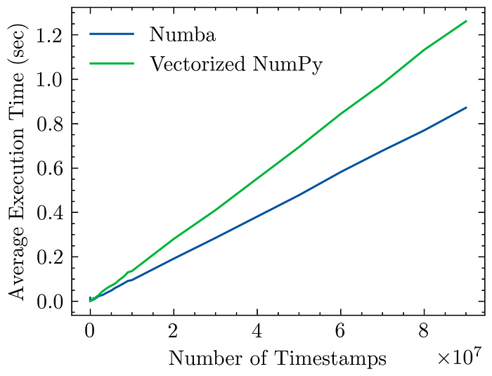
Comparison of Numba and Vectorized NumPy Execution Times’

Interestingly, we observe that Numba effectively speeds up the computation of the profit and loss (PL) even in comparison to the already highly optimized NumPy-vectorized approach.This highlights the compelling advantages of employing Numba for validating short-term parametric models.

A big thank you to all the readers! I truly appreciate your time and interest in this article.

Feel free to contact me at francesco.landolfi@epiphany-alpha.com and subscribe to my medium page to be updated on new pieces on systematic trading related topics.

Linkedin profile: https://www.linkedin.com/in/francesco-landolfi-2311953/

YouTube channel ( if you are not only interested in data science! ) https://www.youtube.com/@FraLandolfi/

More content at PlainEnglish.io.

Sign up for our free weekly newsletter. Follow us on Twitter, LinkedIn, YouTube, and Discord.

---

Validation of Parametric Short-term Strategies with Python: How Fast Can You Really Go? was originally published in Artificial Intelligence in Plain English on Medium, where people are continuing the conversation by highlighting and responding to this story.

https://ai.plainenglish.io/validation-of-parametric-short-term-strategies-with-python-how-fast-can-you-really-go-221b6c4784c6?source=rss—-78d064101951—4
By: Francesco Landolfi
Title: Validation of Parametric Short-term Strategies with Python: How Fast Can You Really Go?
Sourced From: ai.plainenglish.io/validation-of-parametric-short-term-strategies-with-python-how-fast-can-you-really-go-221b6c4784c6?source=rss—-78d064101951—4
Published Date: Fri, 07 Jul 2023 00:42:46 GMT

Did you miss our previous article…
https://e-bookreadercomparison.com/4-ways-to-encode-categorical-features-with-high-cardinality/