Anomaly Detection with BIRCH
Summary
How to Handle High-Dimensional Data with lesser labeled anomalies

Table of contents:
- Introduction
- How Birch works in anomaly detection
- Code for Implementation
- Possible Optimizations and future scope
- References
Introduction:
Anomaly detection is the most widely used AI technique for identifying data patterns that deviate from normal or expected behavior. It is used in various applications in multiple domains, such as fraud detection, network intrusion detection, fault diagnosis, signal processing, and so on. Anomaly detection can help you discover and prevent potential problems and threats before they cause serious damage; along with root cause analysis of asset health management systems.
Tons of algorithms are there. Tons of choices are there. That thing makes the selection of an algorithm more difficult based on specific use cases. Every method comes with many advantages and disadvantages based on different parameters such as sensitivity, computational complexity, lack of interpretability, etc.
Here, I will introduce you to the BIRCH algorithm, which stands for Balanced Iterative Reducing and Clustering using Hierarchies. This unsupervised algorithm is optimized for high performance on large data sets. It can also reduce noise and outliers in the data by merging or splitting clusters based on a threshold parameter. The BIRCH algorithm more is superior to the popular algo k-means clustering algorithm, as it is more optimized in terms of speed, memory usage, and accuracy. The dataset is signal data fetched from sensors with lesser labeled or captured anomalies; birch can be the best choice in such cases.
How the Birch algorithm works for anomaly detection in easy ways:
- Finding the Normal Behavior:
- Birch identifies a group of sensor readings that represent normal behavior.
- This group represents how the sensors typically behave under regular conditions.
- It’s like identifying a baseline or expected behavior for the sensors.
2. Detecting Anomalies:
- Now comes the exciting part! Birch starts looking for deviations from the normal behavior.
- It examines sensor readings that don’t fit into the established groups or clusters.
- These readings are potential anomalies that could indicate something unexpected or abnormal happening.
3. Scoring the Anomalies:
- Birch assigns scores to each potential anomaly based on how far they deviate from normal behavior.
- The greater the deviation, the higher the anomaly score.
- This scoring helps us prioritize and understand the severity of the anomalies.
4. Threshold for Anomalies:
- Finally, we set a threshold to separate anomalies from normal readings.
- Any potential anomaly with a score above the threshold is flagged as an actual anomaly.
- It’s like having a threshold to differentiate between a regular day and a day when something unusual happens.
Code for Implementation:
Here we will generate synthetic code which is similar to any IIOT or sensor data with some anomalies and will try to detect them using Birch Algorithm.
Generate data
This code is to generate anomaly data of three sensors with some anomalies.
Three sensors: sensors 1 , 2 , 3 with 5 min freq for each of one month’s data.
import pandas as pd
import numpy as np
from sklearn.cluster import Birch
from sklearn.preprocessing import StandardScaler
from scipy.spatial import distance
import matplotlib.pyplot as plt

# Generate synthetic dataset
np.random.seed(42)  # For reproducibility

# Set parameters
num_days = 30
num_samples_per_day = int(24 * 60 / 5)  # Number of 5-minute intervals in a day
num_sensors = 3

# Generate timestamps
timestamps = pd.date_range(start='2023-01-01', periods=num_days * num_samples_per_day, freq='5min')

# Generate sensor data
sensor_data = np.random.randn(num_days * num_samples_per_day, num_sensors)
anomaly_indices = np.random.choice(range(num_days * num_samples_per_day), size=10, replace=False)  # Generate 10 random anomaly indices
sensor_data[anomaly_indices] += 5  # Add anomalies to the sensor data

# Create DataFrame from the generated data
df = pd.DataFrame(sensor_data, columns=['sensor1', 'sensor2', 'sensor3'], index=timestamps)
Now, let's view the data frame which is contained.
df.head()

Subplots of each sensor
# Create subplots for each sensor
fig, axes = plt.subplots(nrows=num_sensors, ncols=1, figsize=(12, 8), sharex=True)

# Plot sensor data for each sensor
for i, sensor in enumerate(df.columns):
    axes[i].plot(df.index, df[sensor], label=sensor, color='C{}'.format(i))
    axes[i].set_ylabel('Sensor Value')
    axes[i].legend()

# Set common x-axis label and title
axes[-1].set_xlabel('Timestamp')
fig.suptitle('Sensor Data')

plt.tight_layout()
plt.show()

Now, let’s plot and see the existing anomalies/outliers.
# Plot box plot for each sensor
plt.figure(figsize=(8, 6))
plt.boxplot([df['sensor1'], df['sensor2'], df['sensor3']], labels=['Sensor 1', 'Sensor 2', 'Sensor 3'])
plt.title('Box Plot for Sensor Data')
plt.xlabel('Sensor')
plt.ylabel('Sensor Value')
plt.show()

Applying Birch
# Apply Birch algorithm for anomaly detection
scaler = StandardScaler()
scaled_data = scaler.fit_transform(df.values)

# Set appropriate threshold for anomaly detection
birch = Birch(n_clusters=None, threshold=1.5)
birch.fit(scaled_data)

# Calculate distances to cluster centers
distances = distance.cdist(scaled_data, birch.subcluster_centers_)
min_distances = np.min(distances, axis=1)

# Set threshold to identify anomalies
threshold = np.percentile(min_distances, 99.9)

# Assign anomaly labels
df['anomaly_label'] = np.where(min_distances > threshold, 1, 0)

# Display the dataset with anomaly labels
print(df.head())
print(df.shape)
Understanding the above code:
- We set parameter n_clusters to None to allow the Birch algorithm to adaptively identify clusters based on the characteristics of the data and make it suitable for detecting anomalies without relying on a predetermined number of clusters. This also helps us to focus on only one parameter and that is threshold.
- We can lower the threshold to detect more anomalies.
- Now, clusters have been formed. So, we also have centers of each subcluster. As birch algo creates multiple hierarchical trees; known as clustering feature trees(CFT).
- We find distances from each subcluster’s centroids to the data points. Then we try to find the minimum Euclidian distance among them.
- The choice of percentile (99.9) determines how strict or lenient the threshold is. A higher percentile means a stricter threshold, classifying only the most extreme distances as anomalies using the percentile function. Technically, we are trying to spotlight only 0.01 percent of the outliers as anomalies.
- branching_factor parameter allows you to control the maximum number of subclusters that can be merged in each level of the algorithm. It can impact memory usage and the trade-off between the runtime and clustering quality of the algorithm. we are including this parameter for now to reduce complexity. But, If you need to need with large datasets then this parameter will play the biggest role which avoids the disadvantages of other unsupervised algorithms for anomaly detection.
Detected anomalies
df[(df.anomaly_label == 1)]

Let’s plot anomalies
# Plot anomalies
anomaly_indices = df[df['anomaly_label'] == 1].index

plt.figure(figsize=(12, 6))
plt.plot(df.index, df['sensor1'], label='Sensor 1')
plt.plot(df.index, df['sensor2'], label='Sensor 2')
plt.plot(df.index, df['sensor3'], label='Sensor 3')
plt.scatter(anomaly_indices, df.loc[anomaly_indices, 'sensor1'], color='red', label='Anomalies')
plt.scatter(anomaly_indices, df.loc[anomaly_indices, 'sensor2'], color='red')
plt.scatter(anomaly_indices, df.loc[anomaly_indices, 'sensor3'], color='red')
plt.xlabel('Timestamp')
plt.ylabel('Sensor Value')
plt.title('Sensor Data with Anomalies')
plt.legend()
plt.show()
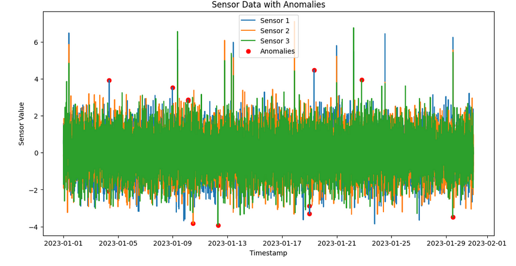
We have successfully detected extreme 0.01% outliers as anomalies.
Possible optimizations and future scope:
There are many possibilities for optimizing the Anomaly detection approach we took in our case apart from parameter tuning:
- Ensembling with different Algos to make the Anomaly detection model more efficient.
- developing better ranking mechanisms to segregate the severity of anomalies.
- Feature engineering to generate new features and use them can increase the efficiency of the model.
I will use and discuss all these techniques in my coming tech articles. Keep me following.
References:
The below article mentions types of data that fit different kinds of clustering or unsupervised approach as per the scenario. It will help you understand this article better way.
G-Means for non-spherical clusters from scratch
Feel free to connect with me on Linkedin , Medium and Topmate.
More content at PlainEnglish.io.
Sign up for our free weekly newsletter. Follow us on Twitter, LinkedIn, YouTube, and Discord.
Anomaly Detection with BIRCH was originally published in Artificial Intelligence in Plain English on Medium, where people are continuing the conversation by highlighting and responding to this story.
https://ai.plainenglish.io/anomaly-detection-with-birch-7f0b5f35ed16?source=rss—-78d064101951—4
By: Abhishek
Title: Anomaly Detection with BIRCH
Sourced From: ai.plainenglish.io/anomaly-detection-with-birch-7f0b5f35ed16?source=rss—-78d064101951—4
Published Date: Wed, 12 Jul 2023 06:17:12 GMT
Did you miss our previous article…
https://e-bookreadercomparison.com/did-you-know-that-chatgpt-is-making-up-facts-just-like-that/