Logistic Regression with PyTorch

Creating a simple classifier model using deep learning workflow.

Intro

Logistic regression is a machine learning model that we can use to perform classification task. In this article, I will explain how I implement a logistic regression model using Pytorch. I used to use Scikit-Learn to do so, and today I want to try implementing it another way. In fact, what we are actually doing here is more similar to a perceptron that uses sigmoid activation function rather than the logistic regression that we know in machine learning. This is due to the fact that we are going to use a workflow that is commonly used for training a deep neural network, yet with only a single neuron. Additionally, I am not going to get deeper into the math behind logistic regression since I will pay more attention to the codes instead.

The structure of this article can be seen below:

1. Creating Dataset
2. Setting up Logistic Regression Model
3. Model Training
4. Evaluation and Visualization

Prior to doing all these steps, let’s import the modules that we need first.

# Codeblock 1
import numpy as np
import torch
import torch.nn as nn
import torch.optim as optim
import matplotlib.pyplot as plt
from sklearn.datasets import make_classification
from sklearn.model_selection import train_test_split

Creating Dataset

The dataset to be used in this project is going to be generated manually. This can be achieved by making use of make_classification() function which is imported from Scikit Learn. This function returns two outputs: an array of samples (X) and the corresponding labels (y).

# Codeblock 2
X, y = make_classification(n_samples=500, n_features=2, n_classes=2, n_informative=2, 
                           n_redundant=0, n_clusters_per_class=1, random_state=100)

The three parameters of the function above that I want to pay attention to is the n_samples, n_features and n_classes which I set to 500, 2 and 2, respectively. The first two arguments basically tell the function to create an array X of 500 rows and 2 columns (500 datapoints and 2 features). Meanwhile, the latter denotes that those 500 datapoints come from two different classes. Below is what the X and y arrays look like.

# Codeblock 3
print(X[:10])

# Codeblock 4
print(y[:10])

Since our dataset consists of two features, hence we can visualize it using a scatterplot. Here we assume that the first feature (column) is going to act as the horizontal axis while the second one will be the vertical axis. Below is the code to do so.

# Codeblock 5
plt.figure(figsize=(7,7))
plt.scatter(X[:,0], X[:,1], c=y, s=10, cmap='rainbow')

The c parameter in the code above tells plt.scatter() to give colors to the datapoints. In this case, the dots drawn in purple are the ones that belong to class 0. You can also see in the above figure that there are several datapoints that apparently do not lie at the correct cluster. And we will just leave them as they are.

Conversion to Pytorch Tensor

The X and y arrays then need to be converted to Pytorch tensor. This is basically done since the Pytorch’s neural network layers are not compatible with Numpy arrays. Below is the code to do so.

# Codeblock 6
X = torch.from_numpy(X).float()
y = torch.from_numpy(y).float().reshape(len(y), 1)

Furthermore, it is important to notice that the labels also need to be reshaped so that it consists of 500 rows and a single column. Again, this is done merely to make the dimension of our tensor compatible with the model.

# Codeblock 7
print(y[:10])

Train Test Split

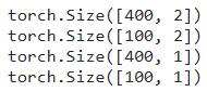
Once we have our dataset in the correct shape, next we will divide it into train and test set. This splitting process is done using train_test_split() with the test ratio of 20%. Since we have 500 datapoints in total, hence the size of the training set is going to be 400 while the rest of those datapoints will be used for testing purpose.

# Codeblock 8
X_train, X_test, y_train, y_test = train_test_split(X, y, test_size=0.2, random_state=999)

print(X_train.shape)
print(X_test.shape)
print(y_train.shape)
print(y_test.shape)

The distribution of those datapoints can be visualized using the code in Codeblock 9. Here I use plus (‘+’) sign to distinguish test data from train data.

# Codeblock 9
plt.figure(figsize=(7,7))
plt.scatter(X_train[:,0], X_train[:,1], c=y_train, s=10, cmap='rainbow')
plt.scatter(X_test[:,0], X_test[:,1], c=y_test, marker='+', s=150, cmap='rainbow')

Setting up Logistic Regression Model

The model that we are going to use is defined in the Logistic_Regression class below.

# Codeblock 10
class Logistic_Regression(nn.Module):
    def __init__(self, num_features):
        super().__init__()
        self.layer0 = nn.Linear(in_features=num_features, out_features=1)
        self.sigmoid = nn.Sigmoid()

    def forward(self, x):
        x = self.layer0(x)
        x = self.sigmoid(x)
        return x

We know that logistic regression is basically a linear equation model in which the resulting output is passed as the argument of a sigmoid function. And the above code does exactly what it supposed to be. I name the linear equation as self.layer0. This layer takes an arbitrary number of input features and outputs a single value. This output is then passed through self.sigmoid layer prior to being returned.

After the Logistic_Regression class have been defined, now that we can use it to initialize the model. Remember that we need to write down the argument of num_features=2 in order to match the model up with our dataset.

# Codeblock 11
model = Logistic_Regression(num_features=2)

In case you’re interested in displaying the model summary, you can use the code shown in Codeblock 12. The output shows that our model consists of 3 params which represents two weights and a single bias.

Note that I do this project using Kaggle Notebook which by default does not include torchinfo module. If you don’t have one either, you can use the install command below to do so prior to actually running the summary() function.

# Codeblock 12
! pip install torchinfo
from torchinfo import summary

summary(model, input_size=X_train.shape)

Model Training

As the dataset and the model have been initialized, now that we will start to work with the training configurations. Here I decided to set the learning rate and the number of training iterations to 0.001 and 4000 respectively.

# Codeblock 13
LEARNING_RATE = 0.001
EPOCHS = 4000

To the loss function, we are going to use binary cross entropy (BCELoss) which the error value will be minimized using SGD (Stochastic Gradient Descent) optimizer. Binary cross entropy is very suitable to be used in a binary classification task. In other cases — typically in multiclass classification tasks, you might need to use CrossEntropyLoss instead.

In the Codeblock 14 below you might also notice that I pass model.parameters() as the first argument for the optimizer. This essentially says that we want the SGD optimizer to update the params of the model — which are basically the 2 weights and a single bias that I mentioned earlier.

# Codeblock 14
loss_function = nn.BCELoss()
optimizer = optim.SGD(model.parameters(), lr=LEARNING_RATE)

I also want to create a function to calculate accuracy score. Later on, this function will be called repeatedly in the training loop so that we can see how the accuracy improves as the training goes.

# Codeblock 15
def calculate_accuracy(preds, actuals):
    
    with torch.no_grad():
        rounded_preds = torch.round(preds)
        num_correct = torch.sum(rounded_preds == actuals)
        accuracy = num_correct/len(preds)
        
    return accuracy

The steps done by the calculate_accuracy() function in Codeblock 15 above is relatively simple. It takes two arrays as the input arguments: prediction results and ground truths. Since the prediction results are still in form of raw values, hence they need to be rounded first so that the resulting value will only be either 0 or 1. This array of rounded values is named rounded_preds. Afterwards, we can simply count the number of matches between the prediction results and the actual labels to get the number of correct predictions. Finally, the resulting value is divided by the total number of predictions to obtain the accuracy score.

Training Loop

The entire training loop is shown in the following code block. The first thing that we need to do here is to initialize empty lists to store the training history. Later on, we are going to make use of those lists to display some graphs.

# Codeblock 16
train_losses = []
test_losses  = []
train_accs = []
test_accs  = []

for epoch in range(EPOCHS):
    # Forward propagation (predicting train data) #a
    train_preds = model(X_train)
    train_loss  = loss_function(train_preds, y_train)
    
    # Predicting test data #b
    with torch.no_grad():
        test_preds = model(X_test)
        test_loss  = loss_function(test_preds, y_test)
        
    # Calculate accuracy #c
    train_acc = calculate_accuracy(train_preds, y_train)
    test_acc  = calculate_accuracy(test_preds, y_test)
    
    # Backward propagation #d
    optimizer.zero_grad()
    train_loss.backward()

    # Gradient descent step #e
    optimizer.step()
    
    # Store training history #f
    train_losses.append(train_loss.item())
    test_losses.append(test_loss.item())
    train_accs.append(train_acc.item())
    test_accs.append(test_acc.item())
    
    # Print training data #g
    if epoch%100==0:
        print(f'Epoch: {epoch} \t|' \
            f' Train loss: {np.round(train_loss.item(),3)} \t|' \
            f' Test loss: {np.round(test_loss.item(),3)} \t|' \
            f' Train acc: {np.round(train_acc.item(),2)} \t|' \
            f' Test acc: {np.round(test_acc.item(),2)}')

Note: Please refer to the letters on the comments (#) as they indicate the specific section of the code that is being discussed.

This training loop is going to iterate according to the number of epochs that we have defined earlier. During a single epoch, there are multiple steps we must take, and the initial step is forward propagation (#a). In this stage, all training samples are predicted by our logistic regression model. It is important to keep in mind that the output of the model (train_preds) is still in form of a float number which lies between 0 and 1 (unrounded) thanks to the nature of a sigmoid function. These unrounded predictions are then compared with the corresponding ground truths (y_train) using our loss_function().

Next, we are going to predict the test data (#b). This step is actually not mandatory since basically the model training will only be done using train data. You’ll also notice that the test data prediction is run inside the torch.no_grad() wrapper. This part of the code is used to tell the program not to keep track of the gradients from the testing samples, as only gradients from training samples are needed to update the network’s params.

In section #c, we will calculate the training and testing accuracy by using the calculate_accuracy() function which we have created previously. The resulting accuracy score will be stored in train_acc and test_acc.

Now here’s the important part. In order to allow our logistic regression model to get trained, we need to perform backpropagation which can be done simply by calling backward() method on our train_loss (#d). This part of the code is going to automatically calculate gradients, in which it will be used for updating the params of our network. The updating process itself is commonly known as gradient descent, and this is done by running optimizer.step() (#e).

The codes in section #f and #g are written for the sake of displaying training progress. Section #f works by appending the loss values as well as the accuracy scores of each epoch. Meanwhile, section #g will show the current training progress every 100 epochs. Below is what the training progress looks like after we run Codeblock 16.

Evaluation and Visualization

After the training has completed, now that we have our training history stored in train_losses, test_losses, train_acc and test_acc. In this part we are going to display them all in form of a graph. The code in Codeblock 17 is used to display how the loss values decrease as the training progresses.

# Codeblock 17
plt.figure(figsize=(10,6))
plt.grid()
plt.plot(train_losses)
plt.plot(test_losses)
plt.legend(['train_losses', 'test_losses'])
plt.xlabel('epoch')
plt.ylabel('loss')
plt.show()

That was the loss value, next we will plot the accuracy score.

# Codeblock 18
plt.figure(figsize=(10,6))
plt.grid()
plt.plot(train_accs)
plt.plot(test_accs)
plt.legend(['train_accs', 'test_accs'])
plt.xlabel('epoch')
plt.ylabel('accuracy')
plt.show()

According to the two graphs above, we can see that the loss value is decreasing and the accuracy score is improving as the training progresses. This indicates that our logistic regression has been trained effectively.

Displaying Decision Boundary

Not only accuracy score, but we can also display the decision boundary generated by our logistic regression classifier. In order to do so, we first need to take the weights and bias of the trained model which later I store those values in param_vector. The Codeblock 19 below shows how I do that. Once again, here also wrap the code using torch.no_grad() since we no longer need to take its gradients.

# Codeblock 19
with torch.no_grad():
    param_vector = torch.nn.utils.parameters_to_vector(model.parameters())
    
print(param_vector)

To be honest it is not quite clear which value in param_vector corrseponds to the first weight, second weight, and the bias. But I found that it is really the sequence after several experiments. With a little bit of math, we can figure out the value for slope (m) and y-intercept (c) so that we can draw a line on a 2D cartesian coordinate system. This is clearly shown in Codeblock 20 section #a.

# Codeblock 20
def show_decision_boundary():
    weight_0 = param_vector[0]
    weight_1 = param_vector[1]
    bias = param_vector[2]
    
    #a
    m = -(bias/weight_1) / (bias/weight_0)
    c = -bias/weight_1

    x_line = np.linspace(X_train[:,0].min(), X_train[:,0].max(), 400)
    y_line = m*x_line + c

    plt.figure(figsize=(7,7))
    plt.scatter(X_train[:,0], X_train[:,1], c=y_train, s=10, cmap='rainbow')
    plt.scatter(X_test[:,0], X_test[:,1], c=y_test, marker='+', s=150, cmap='rainbow')
    plt.plot(x_line, y_line, c='black')

show_decision_boundary()

Once the code above is run, we can see that the decision boundary is able to separate the two classes pretty well. This implies that our logistic regression model is now able to do this binary classification task.

Final words

And that’s it! We have been able create and train a logistic regression model using Pytorch. You can download the notebook that I use through this link.

Thanks for reading!

More content at PlainEnglish.io.

Sign up for our free weekly newsletter. Follow us on Twitter, LinkedIn, YouTube, and Discord.

---

Logistic Regression with PyTorch was originally published in Artificial Intelligence in Plain English on Medium, where people are continuing the conversation by highlighting and responding to this story.

https://ai.plainenglish.io/logistic-regression-with-pytorch-8c3899712fa0?source=rss—-78d064101951—4
By: Muhammad Ardi
Title: Logistic Regression with PyTorch
Sourced From: ai.plainenglish.io/logistic-regression-with-pytorch-8c3899712fa0?source=rss—-78d064101951—4
Published Date: Thu, 27 Jul 2023 04:17:06 GMT

Did you miss our previous article…
https://e-bookreadercomparison.com/ai-builds-momentum-for-smarter-health-care/