TMDB Streamlit : Build Your Own Movie Recommendation System

Understanding Key Concepts and the Science Behind Recommendation Engines while Crafting One from Scratch

Introduction 📌

In the ever-evolving landscape of online platforms like YouTube, Amazon, Netflix, and others, recommender systems have become indispensable in shaping our daily lives. Seamlessly integrated into various facets of our online experiences, these systems play a vital role across e-commerce, online advertising, and media streaming services. Perhaps you’ve explored the vast libraries of Netflix, Prime Video, or YouTube and stumbled upon personalized recommendations for movies and TV shows based on your viewing history or popular trends in your region.

Have you ever pondered the inner workings behind Amazon’s product suggestions, tailored to enhance your shopping journey? Likewise, as a Spotify user, you may have wondered about the behind-the-scenes magic that enables the platform to curate song recommendations aligned with your unique musical preferences.

These remarkable systems are designed to deliver personalized and relevant suggestions, catering to individual user preferences and the characteristics of the items themselves.

In this article, I will guide you through the process of creating a movie recommender system from scratch. We’ll cover essential concepts such as word vectorization and text similarity, providing you with a comprehensive understanding of the underlying principles. Here’s an outline of the topics we will cover 👇

Table of Contents 🔖

1. What are we building ❓
2. Feature Engineering of the Data ⚙️
3. Text Representation and Cosine Similarity 🤝
4. Building Recommendation Engine 🤖
5. Developing web app with Streamlit 🔥

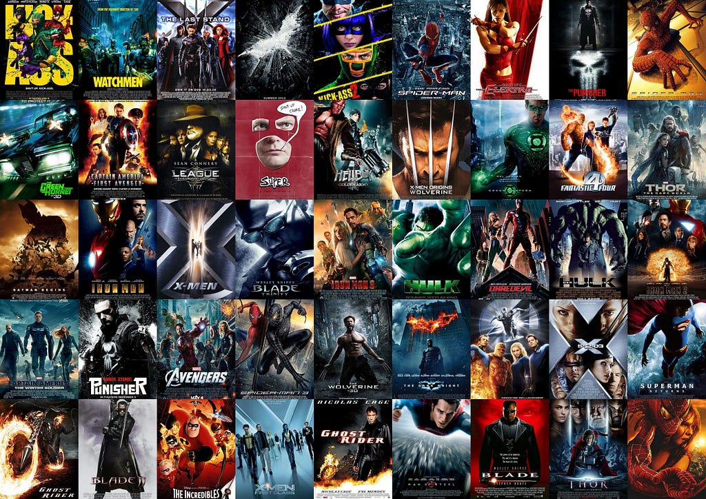
Let’s begin with a glimpse of what awaits at the end of this blog 🍿

If this ignites your motivation, then without a moment’s hesitation, let’s plunge headfirst into our exhilarating adventure 🚀

Section 1: What are we building ?🎯

There are several types of recommendation systems, but we won’t go into detail. Let’s just take a high-level look at some common types of recommendation systems:

Content-based filtering: This approach analyzes item characteristics and user profiles to provide recommendations. It suggests items similar to the ones users have shown interest in, based on shared attributes such as genre or keywords.

Collaborative filtering: By identifying patterns among users or items, collaborative filtering generates recommendations. It looks for similarities between users’ preferences or item ratings to suggest items that others with similar tastes have enjoyed.

Hybrid recommender systems: These systems combine multiple techniques to enhance recommendation accuracy and diversity. They leverage the strengths of different approaches, such as content-based and collaborative filtering, to provide more personalized suggestions.

Knowledge-based systems: Using explicit knowledge and rules, knowledge-based systems make recommendations based on specific criteria or constraints. They incorporate domain knowledge to suggest items that align with predefined rules or user preferences.

Popularity-based systems: These systems rely on the overall popularity of products or items within a particular demographic. Recommendations are based on what is trending or frequently purchased by others.

In addition to these common approaches, specialized recommendation systems are tailored to specific use cases and target audiences. In this article, we will focus on building a content-based recommender engine for movies, where recommendations are based on the type of movies users search for. So, in our next section, let’s dive into exploring and manipulating the content to meet our objectives.

Section 2: Becoming One with the Data 🎬️

To facilitate our project, we will be using the TMDB 5000 dataset available on Kaggle. This dataset contains valuable information about movies, including their titles, genres, keywords, and user ratings. However, before we proceed further, it is essential to perform feature engineering on the dataset. Feature engineering involves transforming and preparing the data to make it suitable for applying machine learning algorithms. By carefully engineering the features, we can extract meaningful insights and ensure the optimal performance of our recommender system.

TMDB 5000 Movie Dataset

Let’s kick off our adventure by acquiring the data from the source. We’ll download and import the necessary libraries, starting with the trusty companion, Pandas. Within this quest, we encounter two CSV files: one that contains credits and another brimming with movie details. Now, I won’t delve too deeply into the intricate nuances of the dataset here, you can readily explore that information from the aforementioned source.

Our ultimate mission is to construct a magnificent DatFrame adorned with movie titles, unique IDs (the magical keys to unlock movie details and posters from IMDB or TMDB), and the cherished corpus of each movie. This magnificent corpus shall encompass all textual treasures that may aid in our noble pursuits of text similarity and recommendation algorithms. Through this feat of feature engineering, we shall craft a dataset of the utmost quality, ready to be expertly processed in the forthcoming realm of Machine Learning.

Coming back to the data exploration, Let’s fire up Jupyter Notebook and load the datasets ⚡

# import deps
import pandas as pd

# load datasets
df_cred = pd.read_csv("tmdb_5000_credits.csv")
df_mov = pd.read_csv("tmdb_5000_movies.csv")

# See the size of data sets
df_cred.shape, df_mov.shape

>>> ((4803, 4), (4803, 20))

Our first step entails merging the two DataFrames together. To accomplish this, we will leverage the common movie ID column present in both DataFrames. However, it’s worth noting that the column names for the movie ID differ between the two DataFrames. Therefore, we will rename the columns accordingly to ensure a seamless merge.

Additionally, it is prudent to verify the consistency and synchronicity of the values before proceeding with the merge. You can run the provided code snippet to perform this essential check.

(df_cred.movie_id != df_mov.id).any().sum()

>>> 0

Now we’ll rename the column movie_id name in df_cred to id followed by merge.

# rename column name
df_cred.rename(columns = {'movie_id':'id'}, inplace = True)

# merge the two dataframes & store in df
df = df_cred.merge(df_mov, on = 'id')

Let’s take a look at the data types of the columns in our DataFrame.

# Lets take a look at the data type of the columns
df.info()

<class 'pandas.core.frame.DataFrame'>
RangeIndex: 4803 entries, 0 to 4802
Data columns (total 23 columns):
 #   Column                Non-Null Count  Dtype  
---  ------                --------------  -----  
 0   id                    4803 non-null   int64  
 1   title_x               4803 non-null   object 
 2   cast                  4803 non-null   object 
 3   crew                  4803 non-null   object 
 4   budget                4803 non-null   int64  
 5   genres                4803 non-null   object 
 6   homepage              1712 non-null   object 
 7   keywords              4803 non-null   object 
 8   original_language     4803 non-null   object 
 9   original_title        4803 non-null   object 
 10  overview              4800 non-null   object 
 11  popularity            4803 non-null   float64
 12  production_companies  4803 non-null   object 
 13  production_countries  4803 non-null   object 
 14  release_date          4802 non-null   object 
 15  revenue               4803 non-null   int64  
 16  runtime               4801 non-null   float64
 17  spoken_languages      4803 non-null   object 
 18  status                4803 non-null   object 
 19  tagline               3959 non-null   object 
 20  title_y               4803 non-null   object 
 21  vote_average          4803 non-null   float64
 22  vote_count            4803 non-null   int64  
 dtypes: float64(3), int64(4), object(16)

Upon careful observation, it becomes evident that certain numerical metrics are irrelevant to our specific use case. Therefore, it is logical to exclude them from our analysis and get a cleaned DataFrame to work with.

Now, focusing on the remaining string columns, we must evaluate their potential in helping us construct a comprehensive corpus of keywords or words that encapsulate the essence of each movie. By combining elements such as the movie title, genre, overview, and cast/crew (if we desire to search based on individuals), we can generate a cohesive representation that will enable us to discover similar movies effectively.

Corpus = Title + Genre + Overview + Cast + Crew

There are a few null columns but we will focus only on our target columns so we will drop those rows from DataFrame where overview is null(3 rows).

# drop null overviews
df.dropna(subset = ['overview'], inplace=True)

# filter out target columns
df = df[['id', 'title_x', 'genres', 'overview', 'cast', 'crew']]

# check new df info
df.info()

<class 'pandas.core.frame.DataFrame'>
Index: 4800 entries, 0 to 4802
Data columns (total 6 columns):
 #   Column    Non-Null Count  Dtype 
---  ------    --------------  ----- 
 0   id        4800 non-null   int64 
 1   title_x   4800 non-null   object
 2   genres    4800 non-null   object
 3   overview  4800 non-null   object
 4   cast      4800 non-null   object
 5   crew      4800 non-null   object
 dtypes: int64(1), object(5) 

Now, it’s time to examine the DataFrame and gain a visual understanding of the data contained within each column. By exploring the target columns, we aim to grasp the essence of the problem statement and devise an approach to generate the desired corpus. This exploration will provide valuable insights, enabling us to align our strategies effectively.

The overview and title columns contain simple string values, which makes them straightforward to handle. On the other hand, the genres, cast, and crew columns follow a similar structure, as they consist of lists of dictionaries. To extract the desired values from each dictionary, we need to define a specific approach. For genres, we can include almost all genres associated with each movie as relevant tags. However, when it comes to the cast, including the entire list would lead to increased variance, so we will only add the top three(you can vary) cast members. Similarly, for the crew, we will focus on directors and producers.

To accomplish this, we have two options: we can create separate functions and apply them individually to each DataFrame column, or we can create a single function that directly generates the desired corpus as a series within the DataFrame. In this case, I have chosen the latter approach. The following code snippet will effectively extract the required values as per our specifications.

# Genres
df.genres[0]
>>> '[{"id": 28, "name": "Action"}, {"id": 12, "name": "Adventure"}, 
      {"id": 14, "name": "Fantasy"}, {"id": 878, "name": "Science Fiction"}]'

' '.join([i['name'] for i in eval(df.genres[0])])
>>> 'Action Adventure Fantasy Science Fiction'

Similarly for Cast and Crew:

# taking top 3 cast
' '.join([i['name'] for i in eval(df_feat.cast[0])[:3]])
>>> 'Sam Worthington Zoe Saldana Sigourney Weaver'

# taking crew (director & producer)
' '.join(list(set([i['name'] for i in eval(df_feat.crew[0]) if i['job']=='Director' or i['job']=='Producer'])))
>>> 'James Cameron Jon Landau'

Let’s consolidate all these functions into a single unified function to generate the desired corpus by iteratively passing the respective columns.

# function to generate corpus
def generate_corpus(overview, genre, cast, crew):
    
    corpus = ""
    
    genre = ' '.join([i['name'] for i in eval(genre)])
    
    cast = ' '.join([i['name'] for i in eval(cast)[:3]])
       
    crew = ' '.join(list(set([i['name'] for i in eval(crew) if i['job']=='Director' or i['job']=='Producer'])))
    
    corpus+= overview + " " + genre + " " + cast + " " + crew
    
    return corpus


corpus = []
for i in range(len(df)):
    corpus.append(generate_corpus(df.iloc[i].overview, df.iloc[i].genres, df.iloc[i].cast, df.iloc[i].crew))


len(corpus)
>>> 4800

# check the corpus
corpus[0]
>>> 'In the 22nd century, a paraplegic Marine is dispatched to the moon Pandora on a unique mission, but becomes torn between 
following orders and protecting an alien civilization. Action Adventure Fantasy Science Fiction Sam Worthington 
Zoe Saldana Sigourney Weaver Stephen Lang Michelle Rodriguez Jon Landau James Cameron'

At this point, we have the option to add this newly created column to our DataFrame and either retain or drop the original columns — this choice is yours to make. In my case, I will opt to drop these columns to streamline and reduce the size of our DataFrame.

# rename the column
df.rename(columns = {'title_x':'title'}, inplace = True)

# drop old columns
df.drop(columns=['genres', 'overview', 'cast', 'crew'], inplace=True)

# add corpus
df['corpus'] = corpus

With this final step completed, we are now prepared to move on to the ML part 🚀

Section 3: Text Representation & Text Similarity 🔁

To enable machine learning algorithms to process text data effectively, the textual information must undergo a transformation into a mathematical form, typically represented as vectors of numbers a.k.a vector space model (VSM), where text units are encoded as numerical vectors.

The task of establishing relationships between texts involves a two-step process. The first step, as we previously discussed, involves text representation, wherein the vectors are generated. Once we have these vectors, the second step is to determine methods for comparing them to measure their similarities or differences.

There are various ways of text representation in machine learning. I have covered a few basic approaches (Label Encoding, One Hot Encoder, Dummies) and the Embeddings here👇

Word Embeddings — Text Representation for Neural Networks

So let's discuss a couple of more representation techniques Bag of Words(BoW) and TF-IDF(this we will be using here).

Bag of Words

This method represents the considered text as a collection of words, disregarding their order and context. It assumes that text belonging to a specific class in the dataset can be characterized by a unique set of words. Essentially, it creates a list of vector arrays for each sentence or corpus, where each word is encoded using a one-hot encoding scheme. The size of the list is determined by the number of unique words in the set, forming a Bag 💼 representation.

If two text pieces share similar words, they are considered to belong to the same class or Bag. By analyzing the words present in a text, one can identify the corresponding class it falls into. Consequently, in this representation, documents with the same words will have their vector representations located close to each other in the vector space.

However, this approach results in a sparse representation, with the majority of vector entries being zeroes. This sparsity can lead to computational inefficiencies in terms of storage, computation, and learning (overfitting). To overcome these limitations, the next method introduced is TF-IDF.

TF-IDF

In the previous text representation techniques all words within a text are considered equally significant, with no distinction of importance. However, to overcome this limitation, the concept of TF-IDF (term frequency–inverse document frequency) emerges. TF-IDF strives to measure the relative importance of a word by comparing its frequency in a specific document to its occurrence across the entire corpus. This approach serves as a widely employed representation scheme in information-retrieval systems, aiding in the extraction of relevant documents from a corpus based on a given text query.

TF (term frequency) measures how often a term or word occurs in a given document and TF of a term t in a document d is given as 👇

IDF (inverse document frequency) measures the importance of the term across a corpus. In computing TF (t), all terms are given equal importance (weightage). IDF weighs down the terms that are very common across a corpus and weighs up the rare terms. IDF of a term t is given as 👇

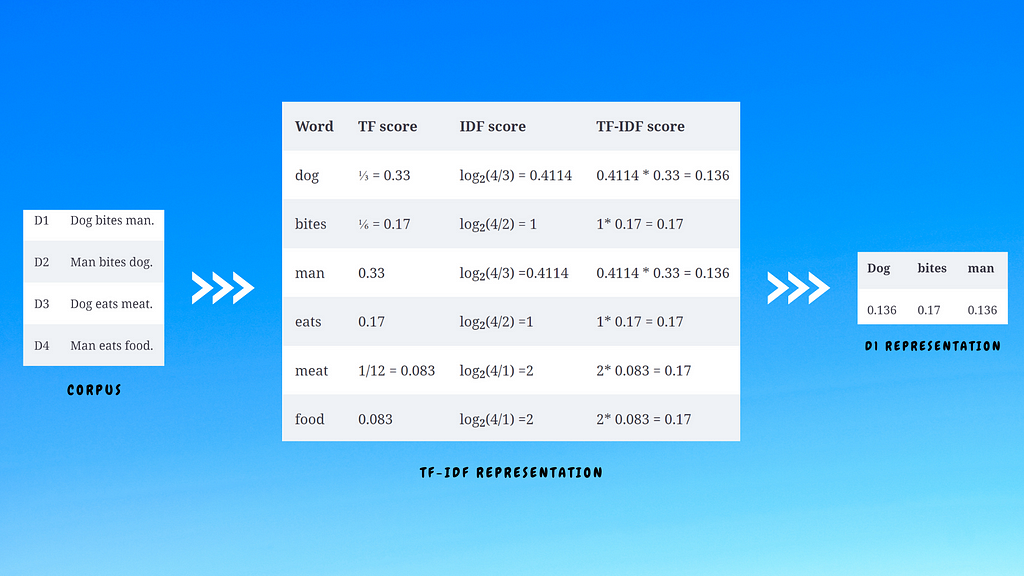
Let’s take an example to understand it better. Here we have a corpus of four documents. The TF-IDF score is calculated for the vocabulary of the corpus(consider the union of unique words across all documents). Then each document is represented as a TF-IDF score of words present to them.

Note: Word preprocessing like stop words removal, stemming , lemmatization is crucial here for the obvious reasons (Ex: Eat, Eating, Eats will all be converted into Eat) hence will lower the dimensions of the array.

We have now converted our text into numerical numbers!! That sounds weird, just envision humans talking with each other in numbers instead of saying Hello 👋 what if someone utters 0.7435 and we instinctively respond with 0.4671 😵‍💫

Alright Alright Alright!!! Coming back to our topic, With the documents represented as vector arrays, what remains is to determine a method for quantifying the similarity between the vector representations. Here are some of the commonly used methods for this purpose 🔗

One of the straightforward yet highly effective techniques for accomplishing this is cosine similarity and we will be using that. Let's do the maths 🧮

Cosine Similarity

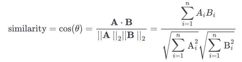
Cosine similarity is a mathematical approach used to measure the similarity between pairs of vectors or rows of numbers treated as vectors. It involves representing each value in a sample endpoint coordinates for a vector, with the other endpoint at the origin of the coordinate system. This process is repeated for two samples, and the cosine between the vectors is computed in an m-dimensional space, where m represents the number of values in each sample. The cosine similarity is such that identical vectors have a similarity of 1 since the cosine of 0 is 1. As the vectors become more dissimilar, the cosine value approaches 0, indicating a lower similarity.

Cosine similarity between two vectors, A and B, each with n components, between them is computed as follows:

The dot product of vectors A (x1​, x2​, x3​) and B (y1​, y2​, y3​), denoted as A.B, can be computed using the following formula:

A.B = x1​∗y1​ + x2​∗y2 ​+ x3​∗y3 ​

and ||A|| & ||B|| is calculated by:

∣∣A∣∣ = ✓(​x1²​+x2​²+x3​²)

∣∣B∣∣ = ✓(​y1²​+y2​²+y3​²)

Let’s consider a simple example in two-dimensional space. It’s worth noting the beauty of mathematics lies in the fact that if we can comprehend a concept in two dimensions, we can extend that understanding to any number of dimensions. Let's walk through the example⚡

# Define three vectors
A = [1, 2]
B = [2, 3]
C = [3, 1]

# Calculate ot products
ab = np.dot(A,B)
bc = np.dot(B,C)
ca = np.dot(C,A)

# calculate the length of the vector
a = np.linalg.norm(A)
b = np.linalg.norm(B)
c = np.linalg.norm(C)

# calculte cosine similarity for each pair using the above formula
sim_ab = ab/(a*b)
sim_bc = bc/(b*c)
sim_ca = ca/(c*a)

# lets see the similarities
sim_ab, sim_bc, sim_ca
>>> (0.9922778767136677, 0.7893522173763263, 0.7071067811865475)

By manually calculating the cosine similarity for each potential pair, we have gained an understanding of the concept. If you find yourself struggling to grasp the concepts, remember the wise words of Andre Ng 🙂

However, in real-life scenarios involving multidimensional data, performing such calculations manually would be a daunting task. Fortunately, scikit-learn (sklearn) comes to the rescue with its convenient solution. By utilizing the pairwise.cosine_similarity class from sklearn, we can effortlessly replicate all these computations with just a single line of code.

# import class
from sklearn.metrics.pairwise import cosine_similarity

# compute cosine similarity
cosine_similarity([A, B, C])

# output
array([[1.        , 0.99227788, 0.70710678],
       [0.99227788, 1.        , 0.78935222],
       [0.70710678, 0.78935222, 1.        ]])

And there we have it! The cosine_similarity function returns a matrix of cosine similarities, similar to a correlation matrix. Each row and column in the matrix represents a vector, resulting in a diagonal matrix where the diagonal values are always one (since the vectors are being compared to themselves).

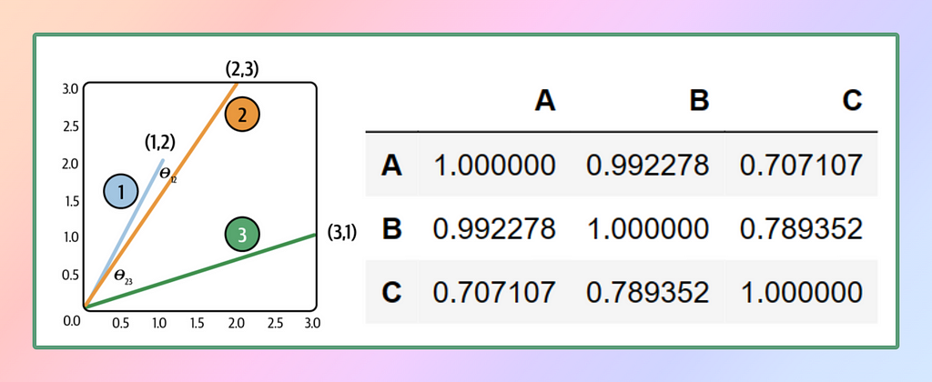
From the obtained results, it becomes apparent that vector A is more similar to vector B compared to vector C. Similarly, vector B is closer to vector C. To gain a visual understanding, let’s plot these vectors in a 2D space and create a DataFrame using the cosine similarity matrix.

DataFrame can be generated using the code:

pd.DataFrame(cosine_similarity(data), 
             columns=['A', 'B', 'C'], 
             index=['A', 'B', 'C'])

Alright, folks, that wraps up the mathematics portion! We’ve dived deep enough into the similarity vectors for foundational understanding but let’s not venture any further, or else we might trigger a cosmic implosion of mathematical proportions! 🙂

So, hoping with our minds still intact, let’s now shift gears ⚙️ and amplify 🚀 this concept upon our movie database.

Section 4: Generating Recommendation Engine 🤖

Next up, we will take the DataFrame we have generated and apply TF-IDF vectorization to the corpus column. This process will yield a feature matrix where the rows represent the movies, and the columns correspond to the textual representations of the vocabulary. We can verify the same via shapes of it.

# import deps
from sklearn.feature_extraction.text import TfidfVectorizer

# Initialize the Object and remove stopwords
tfidf = TfidfVectorizer(stop_words='english')
tfidf_matrix = tfidf.fit_transform(df['corpus'])

# compare shapes
df.shape
>>> (4800, 3)

tfidf_matrix.shape
>>> (4800, 31431)

Now, we have a situation similar to what we previously discussed with examples A, B, and C, in our current context, we have a dataset comprising 4,800 movies, and the text representation of each movie is described by 31,431-word vectors, representing the vocabulary of the entire corpus. To compute the cosine similarity, we need to generate a matrix where the rows and columns represent the 4,800 movies. Each movie will be compared to every other movie along both axes, and their dot product divided by the length of the vectors will yield the cosine similarity values.

Given our prior understanding of the basic example, we can envision the matrix we are aiming to generate. However, to avoid manual calculation, we can leverage the linear kernel provided by scikit-learn. This handy tool simplifies the process of generating the cosine similarity matrix, saving us considerable effort and time.

# import deps
from sklearn.metrics.pairwise import linear_kernel

# compute the similarity matirx
cos_mat = linear_kernel(tfidf_matrix, tfidf_matrix)

cos_mat.shape
>>> (4800, 4800)

It’s astonishingly simple — just a few lines of code, and voila! We have our similarity matrix. As per our theory, the diagonal elements of the matrix should be 1 since each movie is being compared to itself. To verify this, if we sum up all the diagonal elements of the matrix, it should yield a value of 4800. Let’s put it to the test and confirm our expectations!

diag = 0
for i in range(len(cos_mat)):
    diag+= cos_mat[i][i]
    
print(diag)
>>> 4800

Now that we have everything prepared, here’s how the workflow will unfold: When the user provides a movie name, the model will locate the corresponding index of the movie in our DataFrame. We can then use this index to retrieve the same index from the similarity matrix. As the DataFrame and the cosine matrix are aligned, this step yields an array containing the cosine similarity scores of that movie with all other movies in the database.

However, the array is not sorted in any particular order, and we want to showcase the most similar movies. To achieve this, we need to sort the array in descending order. The first element will always correspond to the movie itself, with a similarity score of 1, followed by the other movies in descending order of similarity. Here lies a challenge: Sorting the array will disrupt the original order, making it difficult to fetch the movie titles from the database.

To overcome this, we can store the movie index and similarity score as tuples. Then, we can perform the sorting based on the score alone while keeping the index intact. Subsequently, we can retrieve the movie details using the index from the tuple, ensuring we maintain the correct movie-title association. This approach allows us to obtain the desired similarity rankings while preserving the necessary information for fetching movie details. We can also pass a parameter n for slicing i.e. to fetch top n similar movies. Let’s code it out ⚡

def get_recommendations(movie, n):
    
    # get index from dataframe
    index = df[df['title']== movie].index[0]
    
    # sort top n similar movies     
    similar_movies = sorted(list(enumerate(cos_mat[index])), reverse=True, key=lambda x: x[1]) 
    
    # extract names from dataframe and return movie names
    recomm = []
    for i in similar_movies[1:n+1]:
        recomm.append(df.iloc[i[0]].title)
        
    return recomm


# lets test the function
get_recommendations("The Dark Knight", 3)
>>> ['The Dark Knight Rises', 'Batman Begins', 'Batman Returns']


get_recommendations("Mission: Impossible", 3)
>>> ['Mission: Impossible III',
     'Mission: Impossible II',
     'Mission: Impossible - Ghost Protocol']

And there you have it! We have successfully constructed our very first movie recommendation engine🍿. Congratulations, folks 🎉🎉

Up until now, our movie recommendation system has relied solely on movie names. However, there is a limitation: if a movie name is not present in the DataFrame, or what if a user wants to get recommendations based on cast and crews? our system won’t function as intended. But fear not, for we have a solution at hand! Remember how we incorporated the cast and crew information into the corpus? Well, it’s time to leverage that.

Although the cast and crew details are not directly included in our DataFrame, we can still make use of them. Here’s where TF-IDF comes to the rescue. By applying TF-IDF transformation to the keywords or tags, we can convert them into vectors of the same length as our cosine matrix. And now, you can guess what happens next. Let's walk the talk 🐑

def get_keywords_recommendations(keywords, n):
    
    keywords = keywords.split()
    keywords = " ".join(keywords)
    
    # transform the string to vector representation
    key_tfidf = tfidf.transform([keywords]) 
    
    # compute cosine similarity    
    result = cosine_similarity(key_tfidf, cos_mat)
    
    # sort top n similar movies   
    similar_key_movies = sorted(list(enumerate(result[0])), reverse=True, key=lambda x: x[1])
    
    # extract names from dataframe and return movie names
    recomm = []
    for i in similar_key_movies[1:n+1]:
        recomm.append(df.iloc[i[0]].title)
        
    return recomm

# Let's test it out
get_keywords_recommendations("Christopher Nolan", 4)
>>> ['Insomnia', 'Man of Steel', 'Batman Begins', 'Interstellar']

Wow, the results are truly satisfying, aren’t they? We have successfully achieved our target!

Now, it’s time to switch to the last gear and transition from the notebook environment to a dynamic web application using Streamlit. To utilize the weights from the similarity matrix and the DataFrame effectively, we will save them as binary files using either joblib or pickle.

import joblib

joblib.dump(df, 'models/movie_db.df')
joblib.dump(cos_mat, 'models/cos_mat.mt')
joblib.dump(tfidf, 'models/vectorizer.tf')
joblib.dump(tfidf_matrix, 'models/tfidf_mat.tf')

This way, we can easily load and utilize them within our web application. With these preparations, we bring this section to a fulfilling conclusion.

Section 5: Streaming with Streamlit 🔥

Welcome to the exciting section where creativity knows no bounds! There’s no single perfect way to approach this, and that’s the beauty of it. Streamlit lives up to its reputation of turning data scripts into shareable web apps in minutes, so let’s dive right into it. Brace yourselves, as we’ll cover this section in a flash ⚡

The code for our web app is refreshingly simple and straightforward. We will begin by initializing the binary file, then proceed to obtain user input from a list of movie names using a select box or in the form of text if the user prefers keyword-based recommendations. Based on the input, we will call the appropriate functions to generate the desired recommendations. To keep the app simple, we’ll set the top n parameter to a fixed value of 5.

if search_type == 'Movie Title': 
    st.subheader("Select Movie 🎬")   
    movie_name = st.selectbox('', df.title)
    if st.button('Recommend 🚀'):
        with st.spinner('Wait for it...'):
            movies = get_recommendations(movie_name)
            posters = fetch_poster(movies)        
else:
    st.subheader('Enter Cast / Crew / Tags / Genre  🌟')
    keyword = st.text_input('', 'Christopher Nolan')
    if st.button('Recommend 🚀'):
        with st.spinner('Wait for it...'):
            movies = get_keywords_recommendations(keyword)
            posters = fetch_poster(movies)

To generate picture thumbnails, we will leverage the TMDB API. To access this API, you will need to sign up on TMDB, which typically takes just a couple of minutes. Hers is the link go and signup to generate your free API Key 🗝️

Sign Up – The Movie Database (TMDB)

TMDB has a sweet deal for us with their free API, but there’s a little catch — they just want some love and credit in return. They even kindly provided us with logos to sprinkle all over our application. So get ready to splash those TMDB logos everywhere 😅 Here’s the link for their logos 👇

Logos & Attribution – The Movie Database (TMDB)

The process is fairly straightforward. By fetching the movie details using the movie ID from the DataFrame (which is why we included it in the DataFrame), we will receive a JSON response containing various key-value pairs. Our focus will be on the poster_path key, which provides the URL for the movie poster. We can utilize this URL to display the movie posters in our web application. Here’s what our app will look like 🚀

The entire code for this app can be found in the GitHub repository. You can clone the repository and re-run it to obtain updated weights. Please note that due to GitHub’s file size limit of 100 MB, a reduced dataset will be used to generate the cosine similarity object. However, you can easily run the code on your local machine to achieve the same results. Here’s the repo link 🗃️👇

GitHub – afaqueumer/TMDBAI: Movie Recommendation System using TMDB 5000 Movies Dataset

Conclusion

And here we find ourselves at the conclusion of our never-ending blog! So, my fellow movie aficionados, after all the concepts we’ve absorbed, it’s time to celebrate 🎉🍾🥳 So grab some popcorn🍿 and this time, let’s leave the decision of what to watch 🎬 in the capable hands of our very own app 🍿🤖

I hope you enjoyed this article! and found it informative and engaging. You can follow me Afaque Umer for more such articles.

I will try to bring up more Machine learning/Data science concepts and will try to break down fancy-sounding terms and concepts into simpler ones.

Thanks for reading 🙏Keep learning 🧠 Keep Sharing 🤝 Stay Awesome 🤘

More content at PlainEnglish.io.

Sign up for our free weekly newsletter. Follow us on Twitter, LinkedIn, YouTube, and Discord.

---

🎬 TMDB 🤝 Streamlit 🔥: Build Your Own Movie Recommendation System 🚀 was originally published in Artificial Intelligence in Plain English on Medium, where people are continuing the conversation by highlighting and responding to this story.

https://ai.plainenglish.io/tmdb-streamlit-build-your-own-movie-recommendation-system-f2ffbca63d11?source=rss—-78d064101951—4
By: Afaque Umer
Title: TMDB Streamlit : Build Your Own Movie Recommendation System
Sourced From: ai.plainenglish.io/tmdb-streamlit-build-your-own-movie-recommendation-system-f2ffbca63d11?source=rss—-78d064101951—4
Published Date: Mon, 10 Jul 2023 01:07:49 GMT